Polynomials #
All the gadgets in Plonkbook follow the same high level model, called a polynomial interactive oracle proof (Poly-IOP). Each gadget is defined as an operation on one or more arrays of data. The arrays are encoded into a univariate polynomial (see below) and the polynomial is committed to (next background section) and passed to the verifier. The verifier works with commitments and sees that operations on commitments are mirroring a set of operations being done on the polynomials themselves. And the operations on the polynomials are mirroring operations on the data encoded into them as an array.
Each gadget description will begin with the array and show the operation being done on the array. It will then show how to manipulate a polynomial holding the array so that the operation is performed on the underlying array. It will then show how the verifier can use only commitments to the polynomials, rather than the full polynomials, to follow along and check every step.
Encoding Arrays of Data into Polynomials #
In the Poly-IOP model, data starts as an array (or vector) of integers and gadgets are defined in terms of operations on arrays. In the proof stage, the arrays are encoded into a polynomial. Array slots contain integers between 0 and $q-1$, where $q$ is a large (generally 256 bit) prime number. Recall that we call this set of integers $\mathbb{Z}_q$.
| $\mathsf{data}_0$ | $\mathsf{data}_1$ | $\mathsf{data}_2$ | $\mathsf{data}_3$ | $\mathsf{data}_4$ |
|---|
It is common to denote a polynomial like $P(X)$ where $X$ is the variable of the polynomial. We are going denote the variable with an empty box $\square$ which can be interpreted as a place where you can put any integer in $\mathbb{Z}_q$ you want evaluated (or equivalent, where you place an x-coordinate to learn what the y-coordinate is).
A polynomial in this notation looks like:
- $P(\square)=c_0+c_1\cdot\square+c_2\cdot\square^2+c_3\cdot\square^3+c_4\cdot\square^4=\sum_{i=0}^d c_i\cdot\square^i$
The values $c_i$ are called coefficients. Different arrays of data will (depending on how data is encoded, next) result in different coefficients and thus different polynomials. The degree of the polynomial is the largest exponent. So the polynomial above has degree 4 and thus will have 5 coefficients and 5 terms of the form $c_i\cdot\square^i$ (including $i=0$). Sometimes the coefficient will be zero: the term is thus not written down but in a list of coefficients, it will be included as a 0.
The main question to tackle is how to “encode” an array of integers into a polynomial. This is generally done one of three ways:
- Coefficients
- Evaluation Points
- Roots
Each has its advantages and disadvantages, which we discuss next.
Fast forwarding a bit, once the polynomial is created, it is not shared directly with anyone. Instead, a commitment to it is shared. The commitment does two things: (1) it makes it succinct: e.g., constant size regardless of how long the array is; and (2) it can hide the data in the array as necessary. We will discuss one specific polynomial commitment scheme called KZG. KZG needs the polynomial in the format of a list of its coefficients. If we have the polynomial in a different form, we will have to convert it to coefficients. Thus this needs to be considered when weighing the pros/cons of the three encoding methods.
Encoding 1: Coefficients #
Create polynomial as: $P_1(\square)=\mathsf{data}_0+\square+\mathsf{data}_2\cdot\square^2+\mathsf{data}_3\cdot\square^3+\mathsf{data}_4\cdot\square^4=\sum_{i=0}^d \mathsf{data}_i\cdot\square^i$
Properties:
- Fast 👍: fastest path to commitment as the output is already in coefficient form.
- Addition 👍: two arrays can be added together (slot-by-slot) by simply adding the polynomials together
- Multiplication 👎: no support for multiplication of arrays (Remark: multiplying the polynomials does not multiply the coefficients. It results in a cross multiplication of every term in the first polynomial with every term in the second polynomial. Further the degree of the resulting polynomial will double that of the starting polynomials).
- Opening 🤷🏻: proving the value of the $i$th element in the array is $\mathsf{data}_i$ doing polynomial math on $P_1(\square)$ is not possible. However $\Sigma$-protocols done directly on KZG may enable this kind of proof. In any case, this is not particularly well explored.
- Other useful properties 👍: the sum of all values in a array can be computed by evaluating the polynomial at $P_1(\boxed{1})$! $\sum_{i=0}^d \mathsf{data}_i\cdot\boxed{1}^i=\sum_{i=0}^d \mathsf{data}_i$ . You can also show two arrays have the same sum (called a “sum check”) by subtracting them and showing $P(\boxed{1})=0$.
- Other useful properties 👍: when all coefficients are 0, the polynomial will be the zero polynomial ($P_1(\square)=0$). Coefficients can be entire polynomials, not just integers. A common optimization in Poly-IOP systems is taking a set of equations of polynomials that should equal 0, placing each into the coefficient of a super-polynomial, and showing the super-polynomial is the zero polynomial (which can be proven overwhelmingly by showing it is 0 at a randomly selected point).
Encoding 2: Evaluation Points #
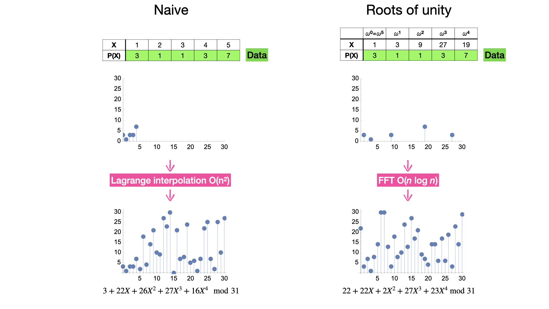
Create a list of points $\{x,y\}$ for the data: $\langle\{0,\mathsf{data}_0\},\{1,\mathsf{data}_1\},\{2,\mathsf{data}_2\},\{3,\mathsf{data}_3\},\{4,\mathsf{data}_4\}\rangle$ and interpolate a polynomial $P_2(\square)$ through these points.
Properties:
- Slow (or moderate) 👎: converting a set of points into a set of coefficients is called interpolation and is $O(n^2)$ time generally. A certain optimization allows $O(n\log n)$ time by choosing $x$ coordinates with a mathematical relationship (more on this later).
- Addition 👍: two arrays can be added together (slot-by-slot) by simply adding the polynomials together
- Multiplication 👍: two arrays can be multiplied together (slot-by-slot) by simply multiplying the polynomials together
- Opening 👍: proving the value of the $i$th element in the array is $\mathsf{data}_i$ is possible with polynomial math by showing $P_2(\boxed{i})=\mathsf{data}_i$ and KZG has a precise algorithm for this.
Encoding 3: Roots #
Create polynomial as: $P_3(\square)=(\square-\mathsf{data}_0)(\square-\mathsf{data}_1)(\square-\mathsf{data}_2)(\square-\mathsf{data}_3)(\square-\mathsf{data}_4)$
Alternatively, create a list of roots $\{x,0\}$ for the data: $\langle\{\mathsf{data}_0,0\},\{\mathsf{data}_1,0\},\{\mathsf{data}_2,0\},\{\mathsf{data}_3,0\},\{\mathsf{data}_4,0\}\rangle$ and interpolate a polynomial $P_3(\square)$ through these points.
Properties:
- Slow 👎 (or moderate): multiplying out naively requires $O(n^2)$ time. Treating as a set of points and interpolating also requires $O(n^2)$ time (because the x-coordinates are the data, they cannot be chosen freely to optimize interpolation). Applying divide and conquer can provide $O(n \log^2 n)$.^[1]
- Addition 👎: two arrays cannot be added from adding (or otherwise manipulating) the polynomials.
- Multiplication 👎: two arrays cannot be multiplied from multiplying (or otherwise manipulating) the polynomials (but you can do a “union” operation below).
- Opening 👍: proving that a value is in the array somewhere is easy and KZG as a precise algorithm for this (opening a root is the same as opening a point, where the y-coordinate is 0). However you cannot show a value is specifically the $i$th value in the array because the polynomial loses the order of the data in the array (see next property).
- Other useful properties 👍: the order of the data in the array does not matter. The same polynomial will be produced even if the order is changed. This is useful when the array represents a “bag” of unordered data. You can easily prove two “bags” of data are the same because the polynomials will be the same. One use-case of this is proving the output of a shuffle/permutation is the same data as the input (just in a different order).
- Other useful properties 👍: multiplying two polynomials results in a concatenation of the data in the arrays (or conjunction/union of the data in both bags). This might be useful in some protocols.
Decision Tree for Encoding #
Basically we decide if we specifically need unordered “bags” of data. If so, encoding as roots is the only option. If not, we consider if we need to ever get the data back from the polynomial. Generally we do and encoding as evaluation points is the most common encoding technique. When do we encode the data and never want it back? Usually when (1) the coefficients are all supposed to be zero so we are just showing that property, or (2) we want back the sum of the data and not the data itself. In these cases, you can still work with evaluation point encoding but it will be faster to just do coefficient encoding.
flowchart LR; A[Array to Polynomial] --> B{Is the data unordered?}; B -- Unordered --> C[Roots]; B -- Ordered or don't care --> D{Open data from polynomial later?}; D -- Yes --> E[Evaluation Points]; D -- No --> F[Coefficients];
The short answer is to start with evaluation point encoding until you realize you need something different.
Roots of Unity #
Moving forward, we will assume we are using Encoding 2: Evaluation Points. In short, this means placing the elements of our array into the $y$-coordinates ($\mathsf{data}_i=P(\boxed{x_i})$) of points on the polynomial. Before commiting to $P(\square)$, we need to use interpolation to find the coefficients of the polynomial that is fitted to these points. General interpolation algorithms are $O(n^2)$ work for $n$ evaluation points but this can be reduced to $O(n\log n)$ with an optimization.
The optimization we will explore enables interpolation via the fast Fourier transform (FFT). It concerns how to choose the $x$-coordinates, which will serve as the index for accessing the data: evaluating $P(X)$ at $x_i$ will reveal $\mathsf{data}_i$. First note, $x$-coordinates are from the exponent group ($Z_q$) and the choices exceed what is feasible to use ($2^{255}$ values in bls). Any subset can be used and interpolated. The optimization is to chose them with a mathematical structure. Specifically, instead an additive sequence (e.g., $0,1,2,3,\ldots$), we use a multiplicative sequence $1,\omega,\omega\cdot\omega,\omega\cdot\omega\cdot\omega,\ldots$ or equivalently: $\omega^0,\omega^1,\omega^2,\ldots,\omega^{\kappa-1}$. Further, the sequence is closed under multiplication which means that next index after $\omega^{\kappa-1}$ wraps back to the first index: $\omega^{k-1} \cdot \omega = \omega^\kappa = \omega^0=1$ (this property is also useful in proving relationships between data in the array and its neighbouring values).
For terminology, we say $\omega$ is a generator with multiplicative order $\kappa$ in $\mathbb{Z}_q$ (or $\omega \in \mathbb{G}_\kappa$). This implies $\omega^\kappa=1$. Rearranging, $\omega=\sqrt[\kappa]{1}$. Thus we can equivalently describe $\omega$ as a $\kappa$-th root of 1. Finally, as 1 is the unity element in $Z_q$, $\omega$ is commonly called a $\kappa$-th root of unity.
For practical purposes, $\kappa$ represents the length of the longest array of data we can use in our protocol. Where does $\kappa$ come from? Different elements of $Z_q$ will have different multiplicative orders but every order must be a divisor of $q-1$. Thus $\kappa$ is the largest divisor of the exact value of $q$ used in an elliptic curve standard. BLS12-384 has $\kappa=2^{32}$ (for terminology, this called a $2$-adicity of $32$). In summary, we can only encode data arrays of length up to $2^{32}=4,294,967,296$.
Interpolation via FFT #
Background #
FFT is a fast algorithm for transitions between coefficients (Encoding 1) and evaluation points (Encoding 2) .
flowchart LR co[coefficients] points[points] co --evaluation--> points points --interpolation--> co
Polynomials, interpolation, and Fourier transforms are all big topics that have general theories and applications. This article will not try to explain anything in its full generality. Instead we will simplify as much as possible, limiting ourselves to only what we need for many cryptographic applications.
Here are the simplifications:
- We only use integers. No real numbers. No imaginary numbers.
- Integers are from a bounded range: $[0,q-1]$ or $\mathbb{Z}_q$ for a large (e.g., 256 bit) prime $q$.
- Polynomials are univariate (only one variable).
Worked Example: Evaluation #
Assume $q=97$.
We will start with the more intuitive direction: going from a polynomial in coefficient form to a set of points on the polynomial. Consider the following polynomial in coefficient form:
$$ P(\square)=81 \square^7+57 \square^6+11 \square^5+59 \square^4+60 \square^3+83 \square^2+45 \square+44 $$In this case, the list of coefficients (from least to greatest) is $\{44,45,83,60,59,11,57,81\}$. The degree of the polynomial is 7 and the number of coefficients is 8. Our goal is determine 8 unique points of form ($x_i, y_i=P(x_i))$. Why 8? We need 8 points to fully determine a degree 7 polynomial, so this will let us reverse the process (go from points to coefficients) in the future if need to.
(Remark: Think of a straight line. It is of form $P(\square)=c_1\square+c_0$ which is degree $1$ with $2$ coefficients. You need $2$ points to figure out what the line should be. Generalizing, for a degree $d$ polynomial, $d+1$ coefficients or $d+1$ points are needed to fully determine it.)
So the goal is to find $8$ points on the polynomial $P(\square)$. The points can be at any x-coordinates so we will chose $\{1,2,3,4,5,6,7,8\}$ for now. We call this the domain. Finding the points is a simple as plugging the x-coordinates into the $P(\square)$ equation:
$$ \begin{alignat}{1} P(\boxed{1})=81 \boxed{1}^7+57 \boxed{1}^6+11 \boxed{1}^5+59 \boxed{1}^4+60 \boxed{1}^3+83 \boxed{1}^2+45 \boxed{1}+44=52 \\ P(\boxed{2})=81 \boxed{2}^7+57 \boxed{2}^6+11 \boxed{2}^5+59 \boxed{2}^4+60 \boxed{2}^3+83 \boxed{2}^2+45 \boxed{2}+44=59 \\ P(\boxed{3})=81 \boxed{3}^7+57 \boxed{3}^6+11 \boxed{3}^5+59 \boxed{3}^4+60 \boxed{3}^3+83 \boxed{3}^2+45 \boxed{3}+44=69 \\ P(\boxed{4})=81 \boxed{4}^7+57 \boxed{4}^6+11 \boxed{4}^5+59 \boxed{4}^4+60 \boxed{4}^3+83 \boxed{4}^2+45 \boxed{4}+44=81 \\ P(\boxed{5})=81 \boxed{5}^7+57 \boxed{5}^6+11 \boxed{5}^5+59 \boxed{5}^4+60 \boxed{5}^3+83 \boxed{5}^2+45 \boxed{5}+44=12 \\ P(\boxed{6})=81 \boxed{6}^7+57 \boxed{6}^6+11 \boxed{6}^5+59 \boxed{6}^4+60 \boxed{6}^3+83 \boxed{6}^2+45 \boxed{6}+44=15 \\ P(\boxed{7})=81 \boxed{7}^7+57 \boxed{7}^6+11 \boxed{7}^5+59 \boxed{7}^4+60 \boxed{7}^3+83 \boxed{7}^2+45 \boxed{7}+44=92 \\ P(\boxed{8})=81 \boxed{8}^7+57 \boxed{8}^6+11 \boxed{8}^5+59 \boxed{8}^4+60 \boxed{8}^3+83 \boxed{8}^2+45 \boxed{8}+44=36 \\ \end{alignat} $$In more succinct form, we are moving between a list of 8 coefficients and a list of 8 points on the polynomial.
$$ \left( \begin{array}{cccccccc} 44 & 45 & 83 & 60 & 59 & 11 & 57 & 81 \\ \end{array} \right) \leftrightarrow \left( \begin{array}{cccccccc} 1 & 2 & 3 & 4 & 5 & 6 & 7 & 8 \\ 52 & 59 & 69 & 81 & 12 & 15 & 92 & 36 \\ \end{array} \right) $$Before figuring out how to go backward, we are going redo the same thing one more time, this time using matrix notation. The equivalent computation we just did is the following:
$$ \left( \begin{array}{cccccccc} \boxed{1}^0 & \boxed{1}^1 & \boxed{1}^2 & \boxed{1}^3 & \boxed{1}^4 & \boxed{1}^5 & \boxed{1}^6 & \boxed{1}^7\\ \boxed{2}^0 & \boxed{2}^1 & \boxed{2}^2 & \boxed{2}^3 & \boxed{2}^4 & \boxed{2}^5 & \boxed{2}^6 & \boxed{2}^7\\ \boxed{3}^0 & \boxed{3}^1 & \boxed{3}^2 & \boxed{3}^3 & \boxed{3}^4 & \boxed{3}^5 & \boxed{3}^6 & \boxed{3}^7\\ \boxed{4}^0 & \boxed{4}^1 & \boxed{4}^2 & \boxed{4}^3 & \boxed{4}^4 & \boxed{4}^5 & \boxed{4}^6 & \boxed{4}^7\\ \boxed{5}^0 & \boxed{5}^1 & \boxed{5}^2 & \boxed{5}^3 & \boxed{5}^4 & \boxed{5}^5 & \boxed{5}^6 & \boxed{5}^7\\ \boxed{6}^0 & \boxed{6}^1 & \boxed{6}^2 & \boxed{6}^3 & \boxed{6}^4 & \boxed{6}^5 & \boxed{6}^6 & \boxed{6}^7\\ \boxed{7}^0 & \boxed{7}^1 & \boxed{7}^2 & \boxed{7}^3 & \boxed{7}^4 & \boxed{7}^5 & \boxed{7}^6 & \boxed{7}^7\\ \boxed{8}^0 & \boxed{8}^1 & \boxed{8}^2 & \boxed{8}^3 & \boxed{8}^4 & \boxed{8}^5 & \boxed{8}^6 & \boxed{8}^7\\ \end{array} \right) \cdot \left( \begin{array}{c} 44 \\ 45 \\ 83 \\ 60 \\ 59 \\ 11 \\ 57 \\ 81 \\ \end{array} \right)= \left( \begin{array}{c} ? \\ ? \\ ? \\ ? \\ ? \\ ? \\ ? \\ ? \\ \end{array} \right) $$Evaluating it:
$$ \left( \begin{array}{cccccccc} 1 & 1 & 1 & 1 & 1 & 1 & 1 & 1 \\ 1 & 2 & 4 & 8 & 16 & 32 & 64 & 31 \\ 1 & 3 & 9 & 27 & 81 & 49 & 50 & 53 \\ 1 & 4 & 16 & 64 & 62 & 54 & 22 & 88 \\ 1 & 5 & 25 & 28 & 43 & 21 & 8 & 40 \\ 1 & 6 & 36 & 22 & 35 & 16 & 96 & 91 \\ 1 & 7 & 49 & 52 & 73 & 26 & 85 & 13 \\ 1 & 8 & 64 & 27 & 22 & 79 & 50 & 12 \\ \end{array} \right) \cdot \left( \begin{array}{c} 44 \\ 45 \\ 83 \\ 60 \\ 59 \\ 11 \\ 57 \\ 81 \\ \end{array} \right)= \left( \begin{array}{c} 52 \\ 59 \\ 69 \\ 81 \\ 12 \\ 15 \\ 92 \\ 36 \\ \end{array} \right) $$Efficiency #
Let’s pause for a moment and think about efficiency. First, consider the matrix: it does not depend on the polynomial values at all. It only depends on the domain (or set of x-values) that you want to evaluate the points at. The domain can be decided ahead of time (e.g., we will always use a domain of 1, 2, 3, …) and then the matrix can be computed at that time. From a protocol perspective, the matrix can be pre-computed and can be shared between operations on polynomials of the same degree.
The multiplication is clearly $O(n^2)$ where $n$ is the number of coefficients/evaluation points. The whole point of FFT to reduce the work to $O(n \cdot \log_2{n})$ and that is it. In a world where efficiency is not a concern, you can just do the above and ignore FFT.
Cryptography #
Moving back to cryptography, imagine you have the polynomial in encrypted (or committed or secret shared) form and this encryption is additively homomorphic. To compute the evaluation points under encryption only involves multiplying in known values from the matrix (which are not secret and depend only on the domain), and then doing additions under encryption. Therefore we can evaluate (and, as you will see below, interpolate) under encryption. Sometimes doing things on the points of a polynomial is simpler than on the polynomials themselves (e.g., multiplying polynomials were you only care about a subset of the points on the polynomial). And vice-versa (rotating an array of values: if encode values into a set of polynomial points, interpolate it, multiply in some constants into the polynomial coefficients, and convert back to points, the array will be rotated).
Jargon #
A matrix with the above form is called a Vandermonde matrix. This process is called a discrete Fourier transform (or DFT). FFT is a special case of DFT and is faster.
Worked Example: Interpolation #
Now assume we have a set of points and want to go backwards to determine the coefficients:
$$ \left( \begin{array}{cccccccc} 1 & 2 & 3 & 4 & 5 & 6 & 7 & 8 \\ 52 & 59 & 69 & 81 & 12 & 15 & 92 & 36 \\ \end{array} \right) \rightarrow \left( \begin{array}{cccccccc} 44 & 45 & 83 & 60 & 59 & 11 & 57 & 81 \\ \end{array} \right) $$Placing the evaluation process into matrix multiplication makes interpolation very easy to understand. We simply move the matrix to the other side of the equation, which involves inverting it. Above, we did the following (coefficients to points):
$$ \left( \begin{array}{cccccccc} 1 & 1 & 1 & 1 & 1 & 1 & 1 & 1 \\ 1 & 2 & 4 & 8 & 16 & 32 & 64 & 31 \\ 1 & 3 & 9 & 27 & 81 & 49 & 50 & 53 \\ 1 & 4 & 16 & 64 & 62 & 54 & 22 & 88 \\ 1 & 5 & 25 & 28 & 43 & 21 & 8 & 40 \\ 1 & 6 & 36 & 22 & 35 & 16 & 96 & 91 \\ 1 & 7 & 49 & 52 & 73 & 26 & 85 & 13 \\ 1 & 8 & 64 & 27 & 22 & 79 & 50 & 12 \\ \end{array} \right) \cdot \left( \begin{array}{c} 44 \\ 45 \\ 83 \\ 60 \\ 59 \\ 11 \\ 57 \\ 81 \\ \end{array} \right)= \left( \begin{array}{c} 52 \\ 59 \\ 69 \\ 81 \\ 12 \\ 15 \\ 92 \\ 36 \\ \end{array} \right) $$To do interpolation (points to coefficients), we move the matrix to the other side of the equation:
$$ \left( \begin{array}{c} 44 \\ 45 \\ 83 \\ 60 \\ 59 \\ 11 \\ 57 \\ 81 \\ \end{array} \right)= \left( \begin{array}{cccccccc} 1 & 1 & 1 & 1 & 1 & 1 & 1 & 1 \\ 1 & 2 & 4 & 8 & 16 & 32 & 64 & 31 \\ 1 & 3 & 9 & 27 & 81 & 49 & 50 & 53 \\ 1 & 4 & 16 & 64 & 62 & 54 & 22 & 88 \\ 1 & 5 & 25 & 28 & 43 & 21 & 8 & 40 \\ 1 & 6 & 36 & 22 & 35 & 16 & 96 & 91 \\ 1 & 7 & 49 & 52 & 73 & 26 & 85 & 13 \\ 1 & 8 & 64 & 27 & 22 & 79 & 50 & 12 \\ \end{array} \right)^{-1} \cdot \left( \begin{array}{c} 52 \\ 59 \\ 69 \\ 81 \\ 12 \\ 15 \\ 92 \\ 36 \\ \end{array} \right) $$Solving the inverse matrix, we arrive at:
$$ \left( \begin{array}{c} 44 \\ 45 \\ 83 \\ 60 \\ 59 \\ 11 \\ 57 \\ 81 \\ \end{array} \right)= \left( \begin{array}{cccccccc} 8 & 69 & 56 & 27 & 56 & 69 & 8 & 96 \\ 50 & 33 & 54 & 3 & 53 & 10 & 57 & 31 \\ 7 & 70 & 8 & 86 & 20 & 39 & 76 & 82 \\ 47 & 89 & 24 & 11 & 90 & 12 & 37 & 78 \\ 85 & 57 & 80 & 34 & 90 & 63 & 71 & 5 \\ 55 & 85 & 43 & 77 & 2 & 67 & 91 & 65 \\ 64 & 11 & 45 & 86 & 44 & 12 & 22 & 7 \\ 73 & 71 & 78 & 64 & 33 & 19 & 26 & 24 \\ \end{array} \right) \cdot \left( \begin{array}{c} 52 \\ 59 \\ 69 \\ 81 \\ 12 \\ 15 \\ 92 \\ 36 \\ \end{array} \right) $$Can we always invert the matrix? The answer is yes, assuming each row of the matrix is unique, which is to say, each evaluation point is unique (no repeats). The complexity analysis is the same as evaluation: the matrix can be pre-computed and the multiplication is $O(n^2)$. The FFT trick will work equally well on this matrix.
Jargon #
This process is called the inverse discrete Fourier transform (or iDFT). If each column of the matrix is taken to be a coefficient list of a polynomial, such polynomials are called Lagrange polynomials.
Speeding up evaluation and interpolation #
Divide-and-conquer #
The high level idea of speeding up both processes is called divide-and-conquer. Recall this equation:
$$ \left( \begin{array}{cccccccc} 1 & 1 & 1 & 1 & 1 & 1 & 1 & 1 \\ 1 & 2 & 4 & 8 & 16 & 32 & 64 & 31 \\ 1 & 3 & 9 & 27 & 81 & 49 & 50 & 53 \\ 1 & 4 & 16 & 64 & 62 & 54 & 22 & 88 \\ 1 & 5 & 25 & 28 & 43 & 21 & 8 & 40 \\ 1 & 6 & 36 & 22 & 35 & 16 & 96 & 91 \\ 1 & 7 & 49 & 52 & 73 & 26 & 85 & 13 \\ 1 & 8 & 64 & 27 & 22 & 79 & 50 & 12 \\ \end{array} \right) \cdot \left( \begin{array}{c} 44 \\ 45 \\ 83 \\ 60 \\ 59 \\ 11 \\ 57 \\ 81 \\ \end{array} \right)= \left( \begin{array}{c} 52 \\ 59 \\ 69 \\ 81 \\ 12 \\ 15 \\ 92 \\ 36 \\ \end{array} \right) $$What if we split this up? For example, say we find the evaluation at $\{1,2,3,4\}$ using the first four coefficients $\{44,45,83,60\}$, then we find the evaluation at $\{5,6,7,8\}$ using the last four coefficients $\{59,11,57,81\}$:
$$ \left( \begin{array}{cccc} 1 & 1 & 1 & 1 \\ 1 & 2 & 4 & 8 \\ 1 & 3 & 9 & 27 \\ 1 & 4 & 16 & 64 \\ \end{array} \right) \cdot \left( \begin{array}{c} 44 \\ 45 \\ 83 \\ 60 \\ \end{array} \right)= \left( \begin{array}{c} 38 \\ 73 \\ 24 \\ 57 \\ \end{array} \right) $$ $$ \left( \begin{array}{cccc} 1 & 5 & 25 & 28 \\ 1 & 6 & 36 & 22 \\ 1 & 7 & 49 & 52 \\ 1 & 8 & 64 & 27 \\ \end{array} \right) \cdot \left( \begin{array}{c} 59 \\ 11 \\ 57 \\ 81 \\ \end{array} \right)= \left( \begin{array}{c} 24 \\ 79 \\ 60 \\ 65 \\ \end{array} \right) $$Next, we need some way to combine $\{38,73,24,57\}$ and $\{24, 79, 60, 65\}$ to generate $\{52,59,69,81,12,15,92,36\}$ (that does not add a bunch more work). Assume we can pull this off, then we can recurse using this trick. Instead of directly computing the above two equations (involving two 4x4 matrices), we can split each of them into 2x2 matrices (for a total of four) using the same process. There is just one problem: there isn’t a simple algorithm for the combine step (faster than just computing the entire original matrix) that is going to work for us.
One parameter we can change #
Reconsider the original problem, moving between coefficients (left) and evaluation points (right):
$$ \left( \begin{array}{cccccccc} 44 & 45 & 83 & 60 & 59 & 11 & 57 & 81 \\ \end{array} \right) \leftrightarrow \left( \begin{array}{cccccccc} 1 & 2 & 3 & 4 & 5 & 6 & 7 & 8 \\ 52 & 59 & 69 & 81 & 12 & 15 & 92 & 36 \\ \end{array} \right) $$We cannot control the coefficients of the polynomial — they are what they are. What the polynomial evaluates to at $\{1,2,3,\ldots\}$ is also what it is, we cannot control it. However the one thing we did get to choose is $\{1,2,3,\ldots\}$ itself (which we call the domain). We can map between coefficients and any domain, assuming there are 8 unique evaluation points. They do not have to be these specific points. So the question is, are there a different set of points that are “nicer” to deal with than $\{1,2,3,\ldots\}$?
The domain shows up in the second column of the matrix:
$$ \left( \begin{array}{cccccccc} 1 & 1 & 1 & 1 & 1 & 1 & 1 & 1 \\ 1 & 2 & 4 & 8 & 16 & 32 & 64 & 31 \\ 1 & 3 & 9 & 27 & 81 & 49 & 50 & 53 \\ 1 & 4 & 16 & 64 & 62 & 54 & 22 & 88 \\ 1 & 5 & 25 & 28 & 43 & 21 & 8 & 40 \\ 1 & 6 & 36 & 22 & 35 & 16 & 96 & 91 \\ 1 & 7 & 49 & 52 & 73 & 26 & 85 & 13 \\ 1 & 8 & 64 & 27 & 22 & 79 & 50 & 12 \\ \end{array} \right) $$What if we make the points (the second column) the same values as the second row of the table: a domain of $\{1,2,4,8,16,32,64,31\}$? In this case, we will get a symmetric matrix which is a little “nicer” than one that is asymmetric. We will show both the matrix (using for evaluation) and its inverse (used for interpolation):
$$ \left( \begin{array}{cccccccc} 1 & 1 & 1 & 1 & 1 & 1 & 1 & 1 \\ 1 & 2 & 4 & 8 & 16 & 32 & 64 & 31 \\ 1 & 4 & 16 & 64 & 62 & 54 & 22 & 88 \\ 1 & 8 & 64 & 27 & 22 & 79 & 50 & 12 \\ 1 & 16 & 62 & 22 & 61 & 6 & 96 & 81 \\ 1 & 32 & 54 & 79 & 6 & 95 & 33 & 86 \\ 1 & 64 & 22 & 50 & 96 & 33 & 75 & 47 \\ 1 & 31 & 88 & 12 & 81 & 86 & 47 & 2 \\ \end{array} \right)= \left( \begin{array}{cccccccc} 32 & 41 & 79 & 38 & 34 & 89 & 74 & 2 \\ 41 & 29 & 45 & 70 & 42 & 46 & 25 & 90 \\ 79 & 45 & 2 & 66 & 43 & 95 & 14 & 44 \\ 38 & 70 & 66 & 2 & 44 & 89 & 60 & 19 \\ 34 & 42 & 43 & 44 & 47 & 25 & 22 & 34 \\ 89 & 46 & 95 & 89 & 25 & 81 & 76 & 81 \\ 74 & 25 & 14 & 60 & 22 & 76 & 15 & 5 \\ 2 & 90 & 44 & 19 & 34 & 81 & 5 & 16 \\ \end{array} \right)^{-1} $$This is nice but once we invert the matrix, is not symmetric any more. Is there a matrix where both the original and its inverse are symmetric? The answer is yes! Consider the domain $\{1,33,22,47,96,64,75,50\}$:
$$ \left( \begin{array}{cccccccc} 1 & 1 & 1 & 1 & 1 & 1 & 1 & 1 \\ 1 & 33 & 22 & 47 & 96 & 64 & 75 & 50 \\ 1 & 22 & 96 & 75 & 1 & 22 & 96 & 75 \\ 1 & 47 & 75 & 33 & 96 & 50 & 22 & 64 \\ 1 & 96 & 1 & 96 & 1 & 96 & 1 & 96 \\ 1 & 64 & 22 & 50 & 96 & 33 & 75 & 47 \\ 1 & 75 & 96 & 22 & 1 & 75 & 96 & 22 \\ 1 & 50 & 75 & 64 & 96 & 47 & 22 & 33 \\ \end{array} \right)= \left( \begin{array}{cccccccc} 85 & 85 & 85 & 85 & 85 & 85 & 85 & 85 \\ 85 & 79 & 70 & 8 & 12 & 18 & 27 & 89 \\ 85 & 70 & 12 & 27 & 85 & 70 & 12 & 27 \\ 85 & 8 & 27 & 79 & 12 & 89 & 70 & 18 \\ 85 & 12 & 85 & 12 & 85 & 12 & 85 & 12 \\ 85 & 18 & 70 & 89 & 12 & 79 & 27 & 8 \\ 85 & 27 & 12 & 70 & 85 & 27 & 12 & 70 \\ 85 & 89 & 27 & 18 & 12 & 8 & 70 & 79 \\ \end{array} \right)^{-1} $$With this new domain and the same coefficients, we can find the evaluation points:
$$ \left( \begin{array}{cccccccc} 1 & 1 & 1 & 1 & 1 & 1 & 1 & 1 \\ 1 & 33 & 22 & 47 & 96 & 64 & 75 & 50 \\ 1 & 22 & 96 & 75 & 1 & 22 & 96 & 75 \\ 1 & 47 & 75 & 33 & 96 & 50 & 22 & 64 \\ 1 & 96 & 1 & 96 & 1 & 96 & 1 & 96 \\ 1 & 64 & 22 & 50 & 96 & 33 & 75 & 47 \\ 1 & 75 & 96 & 22 & 1 & 75 & 96 & 22 \\ 1 & 50 & 75 & 64 & 96 & 47 & 22 & 33 \\ \end{array} \right) \cdot \left( \begin{array}{c} 44 \\ 45 \\ 83 \\ 60 \\ 59 \\ 11 \\ 57 \\ 81 \\ \end{array} \right)= \left( \begin{array}{c} 52 \\ 13 \\ 33 \\ 27 \\ 46 \\ 34 \\ 87 \\ 60 \\ \end{array} \right) $$Or we can find the coefficients, given the evaluation points:
$$ \left( \begin{array}{c} 44 \\ 45 \\ 83 \\ 60 \\ 59 \\ 11 \\ 57 \\ 81 \\ \end{array} \right)= \left( \begin{array}{cccccccc} 85 & 85 & 85 & 85 & 85 & 85 & 85 & 85 \\ 85 & 79 & 70 & 8 & 12 & 18 & 27 & 89 \\ 85 & 70 & 12 & 27 & 85 & 70 & 12 & 27 \\ 85 & 8 & 27 & 79 & 12 & 89 & 70 & 18 \\ 85 & 12 & 85 & 12 & 85 & 12 & 85 & 12 \\ 85 & 18 & 70 & 89 & 12 & 79 & 27 & 8 \\ 85 & 27 & 12 & 70 & 85 & 27 & 12 & 70 \\ 85 & 89 & 27 & 18 & 12 & 8 & 70 & 79 \\ \end{array} \right) \cdot \left( \begin{array}{c} 52 \\ 13 \\ 33 \\ 27 \\ 46 \\ 34 \\ 87 \\ 60 \\ \end{array} \right) $$In summary:
$$ \left( \begin{array}{cccccccc} 44 & 45 & 83 & 60 & 59 & 11 & 57 & 81 \\ \end{array} \right) \leftrightarrow \left( \begin{array}{cccccccc} 1 & 33 & 22 & 47 & 96 & 64 & 75 & 50 \\ 52 & 13 & 33 & 27 & 46 & 34 & 87 & 60 \\ \end{array} \right) $$Two questions:
- How did we find the domain $\{1,33,22,47,96,64,75,50\}$?
- If we use $\{1,33,22,47,96,64,75,50\}$, can we do the divide-and-conquer strategy? Is there a combine function that is workable and efficient for these “nice” matrices?
Generating symmetric matrices #
$\{1,33,22,47,96,64,75,50\}$ is a special form. It is of the form $\{\omega^0,\omega^1,\omega^2,\omega^3,\omega^4,\omega^5,\omega^6,\omega^7\}$ where $\omega=33$. Why 33? The size of the domain is $8$, so we choose 33 because the multiplicative order of $\omega=33$ in $q=97$ is also $8$. Equivalently (in different jargon):
- 33 is a generator that generates a multiplicative subgroup of size 8 (mod 97)
- 33 is an 8-th root of unity of 97
So the trick is setting the $x$-values to be generators of a subgroup of the same size as the number of points/coefficients you have. Here we have 8, so we found a generator of order 8.
Can we find a generator of order 9 or 10 or 11 instead? The answer is no. Only certain sized subgroups exist. What dictates it? The answer is the value of $q$. Once $q$ is chosen, then the sizes of subgroups are locked in. Specifically the sizes available are the divisors of $q-1$. So if we factor $96$, we get $96=2^5\cdot3$. That means we have subgroups of size: $\{1, 2, 3, 4, 6, 8, 12, 16, 24, 32, 48, 96\}$. The value of $q$ for cryptography depends on the elliptic curve used. Something like $\texttt{bls12-381}$ uses a $q$ that purposefully has lots of subgroups: $\{2,4,8,\ldots,2^{32}\}$.
The idea is that you find the degree of your polynomial $d$, then you need $d+1$ coefficients/points to represent it, and then you round $d+1$ up to the nearest power of 2 as necessary. The leading coefficients are set to 0.
Revisiting divide-and-conquer #
The remaining question is whether we can split the matrices into smaller (halve) matrices, and then combine the results. The answer is yes if the domain is based on roots of unity (for completeness, the answer is not necessarily no for other kinds of domains, but we do not explore that here).
Recall, with the new domain, we have:
$$ \left( \begin{array}{cccccccc} 44 & 45 & 83 & 60 & 59 & 11 & 57 & 81 \\ \end{array} \right) \leftrightarrow \left( \begin{array}{cccccccc} 1 & 33 & 22 & 47 & 96 & 64 & 75 & 50 \\ 52 & 13 & 33 & 27 & 46 & 34 & 87 & 60 \\ \end{array} \right) $$Instead of dividing the coefficients into the first half and second halves, we will divide them into even coefficients (coefficients of terms $x^i$ where $i$ is even, including 0) and odd coefficients. We treat these two sets of coefficients as new polynomials $P_\mathsf{even}(\square)$ and $P_\mathsf{odd}(\square)$. Then we combine the two based on the following property:
$$ P(\square)=P_{\mathsf{even}}(\square^2)+\square\cdot P_{\mathsf{odd}}(\square^2) $$How does this save computation? We compute the following values:
$$ \begin{alignat}{1} P_\mathsf{even}(\boxed{\omega^0}^2)=P_\mathsf{even}(1)=57 \boxed{1}^3+59 \boxed{1}^2+83 \boxed{1}^1+44=49 \\ P_\mathsf{even}(\boxed{\omega^1}^2)=P_\mathsf{even}(22)=57 \boxed{22}^3+59 \boxed{22}^2+83 \boxed{22}^1+44=72 \\ P_\mathsf{even}(\boxed{\omega^2}^2)=P_\mathsf{even}(96)=57 \boxed{96}^3+59 \boxed{96}^2+83 \boxed{96}^1+44=60 \\ P_\mathsf{even}(\boxed{\omega^3}^2)=P_\mathsf{even}(75)=57 \boxed{75}^3+59 \boxed{75}^2+83 \boxed{75}^1+44=92 \\ \hline P_\mathsf{odd}(\boxed{\omega^0}^2)=P_\mathsf{odd}(1)=81\boxed{1}^3+11\boxed{1}^2+60\boxed{1}^1+45=3 \\ P_\mathsf{odd}(\boxed{\omega^1}^2)=P_\mathsf{odd}{(22})= 81\boxed{22}^3+11\boxed{22}^2+60\boxed{22}^1+45=57 \\ P_\mathsf{odd}(\boxed{\omega^2}^2)=P_\mathsf{odd}(96)=81\boxed{96}^3+11\boxed{96}^2+60\boxed{96}^1+45=12 \\ P_\mathsf{odd}(\boxed{\omega^3}^2)=P_\mathsf{odd}(75)=81\boxed{75}^3+11\boxed{75}^2+60\boxed{75}^1+45=11 \\ \end{alignat} $$We are not done, we have to figure out what to do with these 8 values still. But before showing that, note that while we are performing 8 evaluations, the evaluations only have 4 coefficients, so this is half the work of not using divide-and-conquer. Further, through recursion, we will be halving this over and over again anyways.
Also note that $P_\mathsf{even}(\boxed{\omega^0}^2)=P_\mathsf{even}(\boxed{\omega^4}^2)$ (or the multiplicative order of $\omega^2$ is half of $\omega$) which is why we only need to evaluate the first 4 values.
To combine these values, we take the output of the even evaluations: $\{49, 72, 60, 92\}$ and repeat it: $E=\{49, 72, 60, 92,49, 72, 60, 92\}$. We do the same with odd: $O=\{3, 57, 12, 11,3, 57, 12, 11\}$. We then compute: $E+O\cdot\mathsf{domain}$ (where multiplication is element-wise):
$$ \{49, 72, 60, 92,49, 72, 60, 92\}+(\{3, 57, 12, 11,3, 57, 12, 11\}\cdot\{1,33,22,47,96,64,75,50\})\\ =\{52, 13, 33, 27, 46, 34, 87, 60\} $$That completes the operation and we have.
$$ \left( \begin{array}{cccccccc} 44 & 45 & 83 & 60 & 59 & 11 & 57 & 81 \\ \end{array} \right) \leftrightarrow \left( \begin{array}{cccccccc} 1 & 33 & 22 & 47 & 96 & 64 & 75 & 50 \\ 52 & 13 & 33 & 27 & 46 & 34 & 87 & 60 \\ \end{array} \right) $$Footnotes #
^[1]: Hat tip Pratyush Mishra for suggesting a state-of-the-art algorithm.